Computing the gradient

Now that we are familiar with the backpropagation algorithm as well as the notion of gradient decscent, we can address more technical questions. Questions like, how do we actually compute this gradient? As you know, our model does not have the liberty of visualizing the loss landscape, and picking out a nice path of descent. In fact, our model cannot tell what is up, or what is down. All it knows, and will ever know, is numbers. However, as it turns out, numbers can tell a lot!

Let's reconsider our simple perceptron model to see how we can backpropagate its errors by computing the gradient of our loss function, J(θ), iteratively:

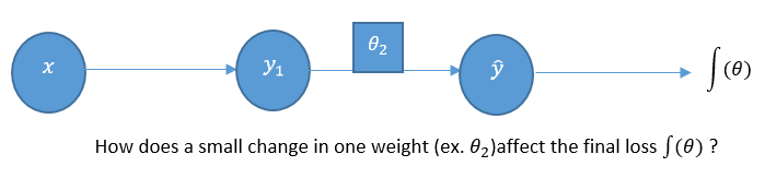
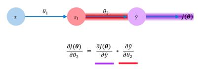
What if we wanted to see how changes in the weights of the second layer impact the changes in our loss? Obeying the rules of calculus, we can simply differentiate our loss function, J(θ), with respect to the weights of the second layer (θ₂). Mathematically, we can actually represent this in a different manner as well. Using the chain rule, we can show how changes in our loss with respect to the second layer weights are actually a product of two different gradients themselves. One represents the changes in our losses with respect to the model's prediction, and the other shows the changes in our model's prediction with respect to the weights in the second layer. This may be represented as follows:

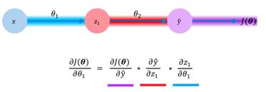
As if this wasn't complicated enough, we can even take this recursion further. Let's say that instead of modeling the impact of the changing weights of the second layer (θ₂), we wanted to propagate all the way back and see how our loss changes with respect to the weights of our first layer. We then simply redefine this equation using the chain rule, as we did earlier. Again, we are interested in the change in our model's loss with respect to the model weights for our first layer, (θ₁). We define this using the product of three different gradients; the changes in our loss with respect to output, changes in our output with respect to our hidden layer value, and finally, the changes in our hidden layer value with respect to our first layer weights. We can summarize this as follows:

And so, this is how we use the loss function, and backpropagate the errors by computing the gradient of our loss function with respect to every single weight in our model. Doing so, we are able to adjust the course of our model in the right direction, being the direction of the highest descent, as we saw before. We do this for our entire dataset, denoted as an epoch. And what about the size of our step? Well, that is determined by the learning rate we set.